
Probabilistic and Reinforcement Learning Track
2023 International Planning Competition
2023 International Planning Competition
XADD Compilation of CPFs
XADD (eXtended Algebraic Decision Diagram) [Sanner at al., 2011] enables compact representation and operations with symbolic variables and functions. In fact, this data structure can be used to represent CPFs defined in a RDDL domain once it is grounded for a specific RDDL instance.
We use the xaddpy package that provides a Pure Python implementation of XADD (originally implemented in Java). To install the package, simply run the following:
pip install xaddpy
In this article, we are going to walk you through how you can use xaddpy to compile a CPF of a grounded fluent into an XADD node.
For example, let’s look at the Wildfire domain and the instance file provided here which has 3 x 3 locations.
Once the CPFs are grounded for this instance, we can see that the values of the non-fluents will simplify the CPFs. For instance, the neighboring cells of the (x1, y1) location are (x1, y2), (x2, y1), and (x2, y2); hence, burning'(x1, y1) should only depend on the states of these neighbors — plus (x1, y1) itself — but none others.
Once you compile the CPFs of this instance into an XADD, you can actually see this structure easily. In other words, XADD compilation reveals the DBN dependency structures of different variables, which we also explain in a separate article.
To run the XADD compilation, we first need to import the domain and instance files. Then, we instantiate the RDDLModelXADD class with the grounded CPFs given by the RDDLGrounder object.
Specifically,
from pyRDDLGym.Examples.ExampleManager import ExampleManager
from pyRDDLGym.Core.Grounder.RDDLGrounder import RDDLGrounder
from pyRDDLGym.XADD.RDDLModelXADD import RDDLModelWXADD
from pyRDDLGym.Core.Parser.RDDLReader import RDDLReader
from pyRDDLGym.Core.Parser.parser import RDDLParser

# Read the domain and instance files
domain, instance = 'Wildfire', '0'
env_info = ExampleManaget.GetEnvInfo(domain)
domain = env_info.get_domain()
instance = env_info.get_instance(instance)

# Read and parse domain and instance
reader = RDDLReader(domain, instance)
domain = reader.rddltxt
parser = RDDLParser(None, False)
parser.build()

# Parse RDDL file
rddl_ast = parser.parse(domain)

# Ground domain
grounder = RDDLGrounder(rddl_ast)
model = grounder.Ground()
From the last line, we get an instance of pyRDDLGym.Core.Compiler.RDDLModel class. Then, we can instantiate a pyRDDLGym.XADD.RDDLModelXADD object:
# XADD compilation
model_xadd = RDDLModelWXADD(model)
model_xadd.compile()
When we call model_xadd.compile(), it will go through each and every CPF of the instance and convert the arithmetic/logical/stochastic/… expressions into an XADD node. Then, you can access the resulting nodes from model_xadd.cpfs, which is a dictionary that maps a grounded fluent name to the integer ID of the corresponding XADD node.
You can print out the node if you do the following:
cpf_burning_x1_y1 = model_xadd.cpfs["burning_x1_y1'"]
model_xadd.print(cpf_burning_x1_y1)
Output:

([put_out_x1_y1]
	 ( [False] )
	 ( [out_of_fuel_x1_y1]
		 ( [burning_x1_y1]
			 ( [True] )
			 ( [False] ))
		 ( [burning_x1_y1]
			 ( [True] )
			 ( [burning_x1_y2]
				 ( [burning_x2_y1]
					 ( [burning_x2_y2]
						 ( [#_UNIFORM_0 - 0.182425523806356 <= 0]
							 ( [True] )
							 ( [False] ) )
						 ( [#_UNIFORM_0 - 0.0758581800212435 <= 0]
							 ( [True] )
							 ( [False] ) )  )
					 ( [burning_x2_y2]
						 ( [#_UNIFORM_0 - 0.0758581800212435 <= 0]
							 ( [True] )
							 ( [False] ) )
						 ( [#_UNIFORM_0 - 0.0293122307513563 <= 0]
							 ( [True] )
							 ( [False] ) )  )  )
				 ( [burning_x2_y1]
					 ( [burning_x2_y2]
						 ( [#_UNIFORM_0 - 0.0758581800212435 <= 0]
							 ( [True] )
							 ( [False] ) )
						 ( [#_UNIFORM_0 - 0.0293122307513563 <= 0]
							 ( [True] )
							 ( [False] ) )  )
					 ( [burning_x2_y2]
						 ( [#_UNIFORM_0 - 0.0293122307513563 <= 0]
							 ( [True] )
							 ( [False] ) )
						 ( [#_UNIFORM_0 - 0.0109869426305932 <= 0]
							 ( [True] )
							 ( [False] )  )  )  )  )  )  )  )
Here, #_UNIFORM_{number} is a special variable that we have introduced to handle random variables. In the Wildfire domain, the burning event follows a Bernoulli distribution, which can be encoded with a random draw from uniform(0, 1) distribution.
A better way to interpret the resulting XADD may be to visualize it as a graph.
You can do this by calling the save_graph method of the XADD object.
context = model_xadd._context   # The XADD object that stores all XADD nodes
context.save_graph(model_xadd.cpfs["burning_x1_y1'"], file_name="burning_x1_y1")
Here’s the result:
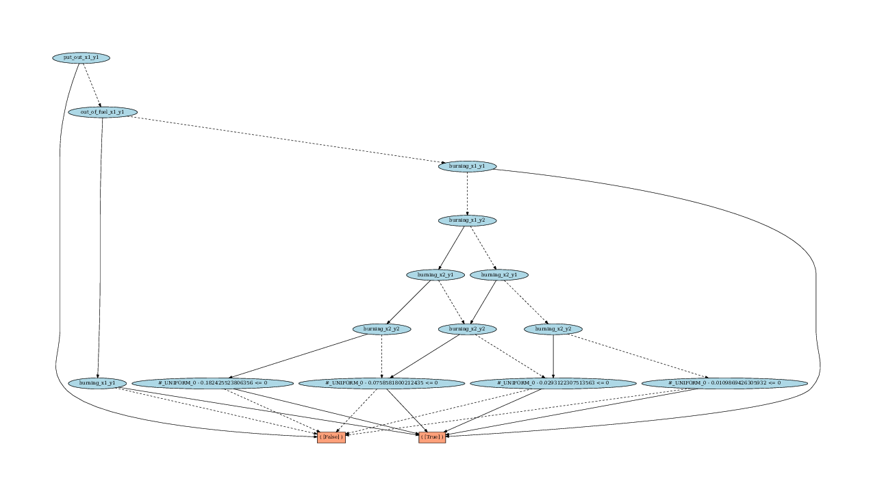
If the figure is too small to comprehend, you can click the link above to check out the XADD graph.
How will the graph look like for out-of-fuel'(x1, y1) variable? Here’s the result of context.save_graph(model_xadd.cpfs["out-of-fuel_x1_y1'"], file_name="out_of_fuel_x1_y1"):
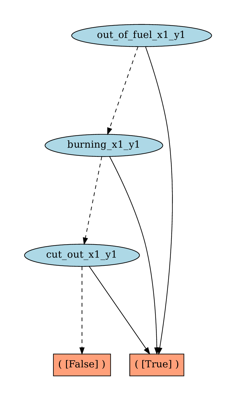
Very neat!
Although the Wildfire example nicely shows how XADD can be used to represent the CPFs of the domain, it only contains Boolean variables. In this part, we will show another example domain that has continuous fluents.
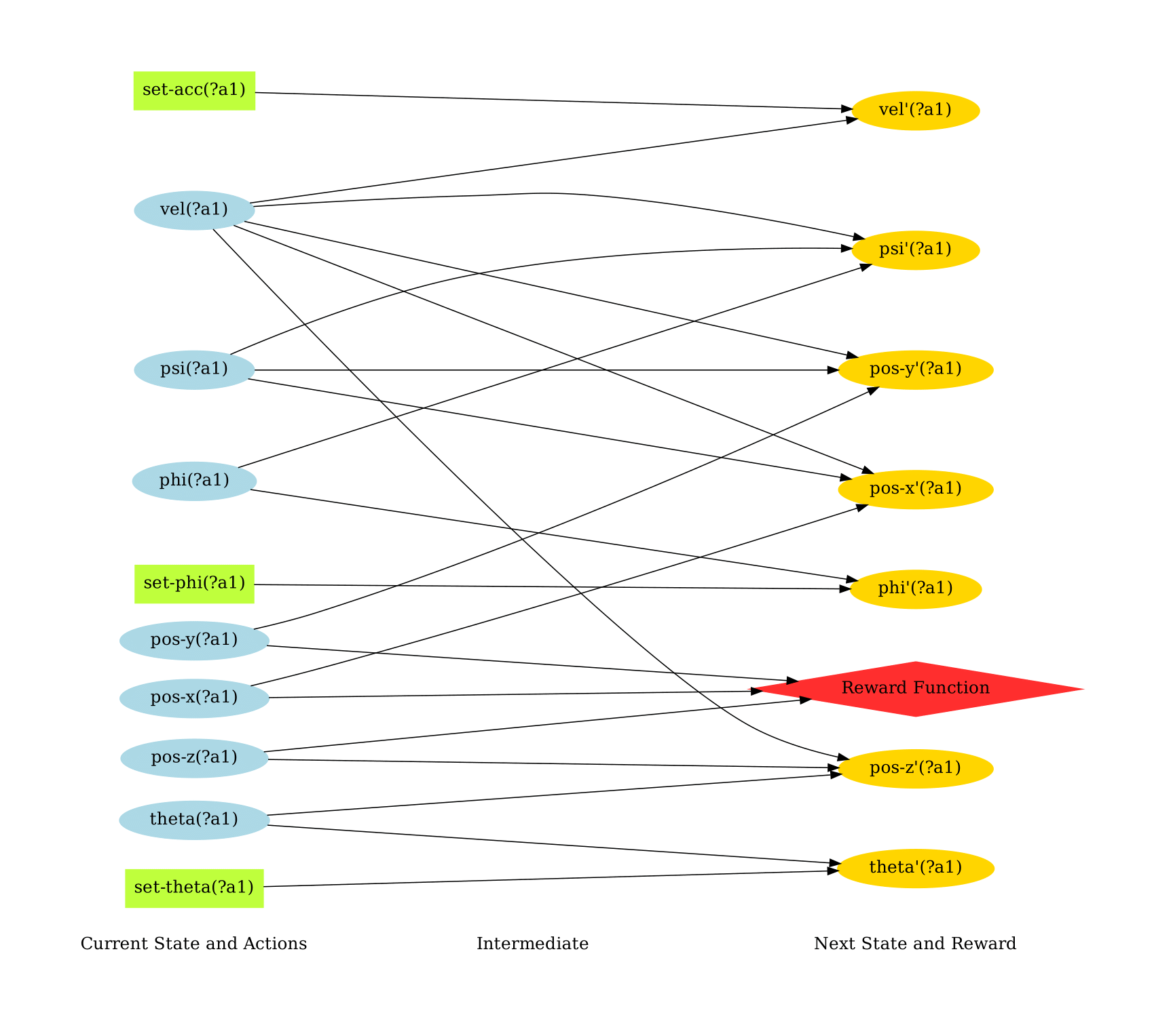
The domain we want to look at is the UAV mixed domain and the instance file is provided here.
If we follow the same procedure described above for the Wildfire domain with the domain name being replaced by 'UAV mixed', then we can compile the domain/instance in XADD. The overall DBN (dynamic Bayes net) structure of this instance is shown below.
Specifically, let’s print out the CPF of vel'(?a1), which is
( [set_acc_a1 - 1 <= 0]
        ( [set_acc_a1 + 1 <= 0]
                ( [vel_a1 - 0.1 <= 0]
                        ( [0] )
                        ( [vel_a1 - 0.1] )
                )
                ( [1.0*set_acc_a1 + 10.0*vel_a1 <= 0]
                        ( [0] )
                        ( [0.1*set_acc_a1 + vel_a1] )
                )
        )
        ( [vel_a1 + 0.1 <= 0]
                ( [0] )
                ( [vel_a1 + 0.1] )
        )
)
When visualized with pygraphviz, we get the following:
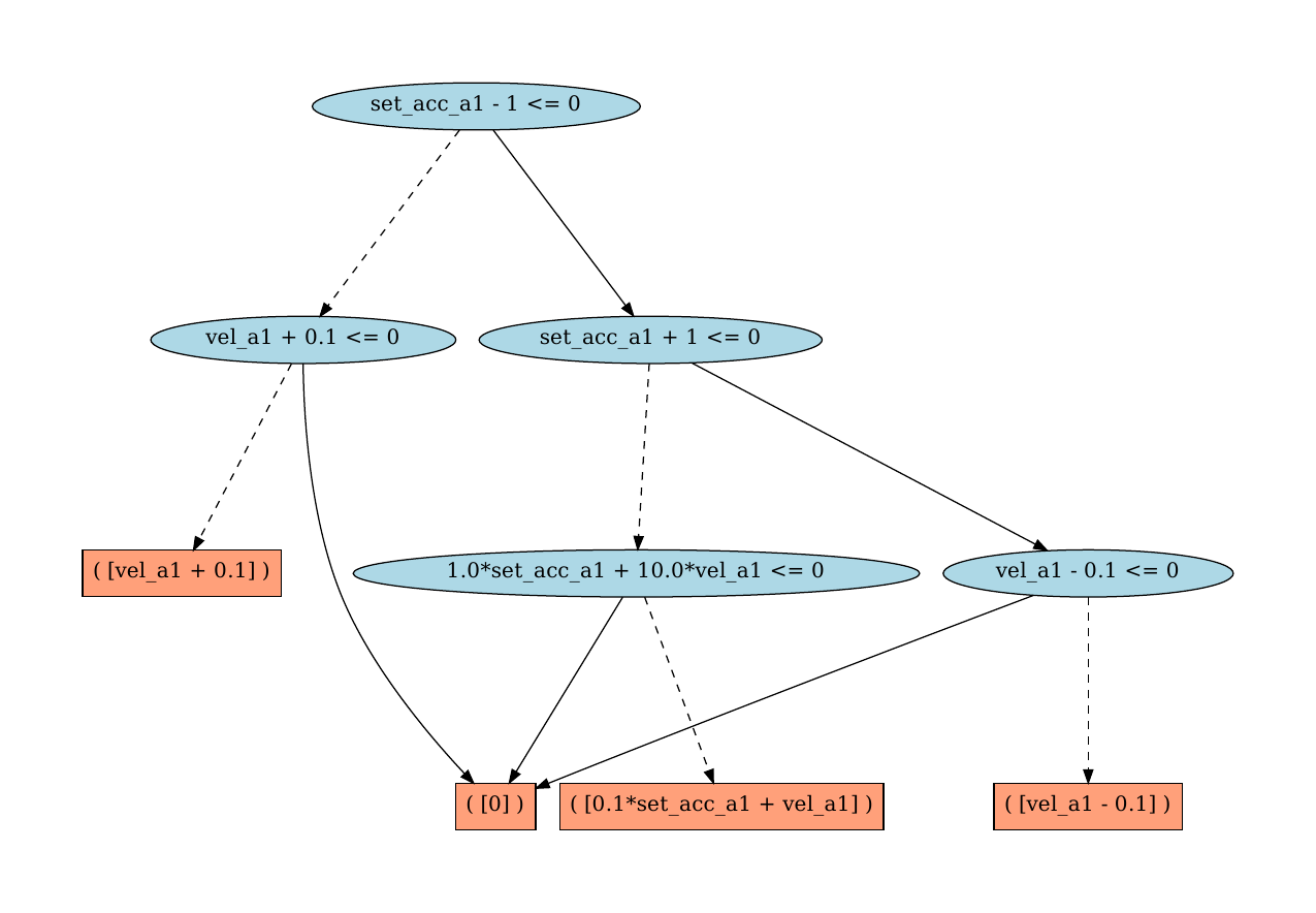
In this case, you can see that the decision nodes have linear inequlity expressions instead of a Boolean decision. As for the function values at the leaf nodes, they are also linear expressions. xaddpy package can also handle arbitrary nonlinear decisions and function values using SymPy under the hood.
Now, you can go ahead and use this functionality to analyze a given RDDL instance!