Visualizing DBNs (Dynamic Bayes Nets) with XADD

With the XADD compilation of a given domain instance, you can easily visualize the dependencies between different fluents. For this purpose, you can use the provided visualization tool that gives you a way to produce diagrams similar to an influence diagram.

Specifically, you can use the pyRDDLGym/Visualizer/visualize_dbn.py file. In this page, we will take you through how to use this file for nicely visualizing a RDDL domain instance.

To begin with, you need to install the following:

1. graphviz
2. pygraphviz
3. xaddpy

Make sure you have activate the right conda environment with conda activate YOUR_CONDA_ENVIRONMENT. Now, we give a step-by-step guide to installing the necessary packages.

Step 1: Installing graphviz

1. For Ubuntu/Debian users, run the following command.

sudo apt-get install graphviz graphviz-dev

1. For Fedora and Red Hat systems, you can do as follows.

sudo dnf install graphviz graphviz-devel

1. For Mac users, you can use brew to install graphviz.

brew install graphviz

Unfortunately, we do not provide support for Windows systems, though you can refer to the pygraphviz documentation for information.

Step 2: Installing pygraphviz

1. Linux systems

pip install pygraphviz

1. MacOS

python -m pip install \
    --global-option=build_ext \
    --global-option="-I$(brew --prefix graphviz)/include/" \
    --global-option="-L$(brew --prefix graphviz)/lib/" \
    pygraphviz

Note that due to the default installation location by brew, you need to provide some additional options for pip installation.

Step 3: Installing xaddpy

XADD (eXtended Algebraic Decision Diagram) [Sanner at al., 2011] enables compact representation and operations with symbolic variables and functions. In fact, the data structure can be used to represent CPFs defined in a RDDL domain once it is grounded for a specific RDDL instance. You can find more detailed description of the XADD compilation step in this page.

We use the xaddpy package that provides a Pure Python implementation of XADD (originally implemented in Java). To install the package, simply run the following:

pip install xaddpy

Visualizing DBNs with XADD

With the necessary tools being installed, we can now go ahead and draw DBN diagrams of various RDDL domain/instances. As a running example, we show how you can visualize a Wildfire instance as defined in pyRDDLGym/Examples/Wildfire.

Instantiate RDDL2Graph object

Firstly, you can instantiate a RDDL2Graph object by specifying the domain, instance, and some other parameters.

from pyRDDLGym.Visualizer.visualize_dbn import RDDL2Graph

r2g = RDDL2Graph(
    domain='Wildfire',
    instance=0,
    directed=True,
    strict_grouping=True,
)

Then, you can visualize the corresponding DBN by calling

r2g.save_dbn(file_name='Wildfire')

which will save a file named Wildfire_inst_0.pdf to ./tmp/Wildfire. Additionally, you can check the Wildfire_inst_0.txt file which records grounded fluent names and their parents in the DBN.

The output of the function call looks like this (opens a new tab showing the PDF file, which we omit to include here since it would take up quite some space).

You can also specify a single fluent and/or a ground fluent that you are interested in for visualization. For example,

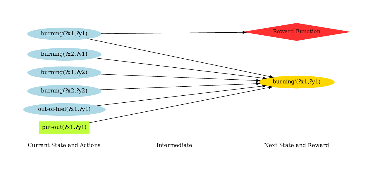
r2g.save_dbn(file_name='Wildfire', fluent='burning', gfluent='x1_y1')

will output the following graph.

huh, Nice! You can see from this diagram that the next state transition of the burning state at (x1, y1) only depends on 6 grounded variables (i.e., whether neighboring cells are burning; whether this location is out of fuel; whether the put-out action has been taken).

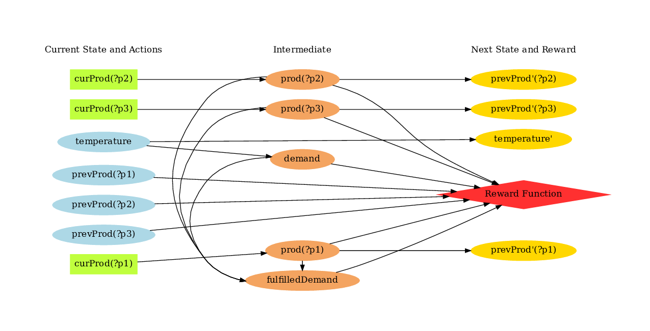
To give you a taste of another example, here’s the DBN visualization of the Power Generation instance, in which intermediate variables are placed in the middle column:

---

Back to main page